Note
Go to the end to download the full example code.
Mass calibration#
This tutorial demonstrates how to estimate a contrast-to-mass calibration from a calibration movie:
Load a calibration movie.
Run detection + PSF fitting to obtain a table of event contrasts.
Fit peaks in the contrast histogram.
Fit a (linear) contrast-to-mass calibration and plot the result.
Imports#
We first import necessary packages and modules.
import matplotlib.pyplot as plt
import numpy as np
Download example data#
This tutorial expects a calibration movie. For now, the example downloads a small calibration file from Zenodo. You can replace this block with a direct file path once you have a local calibration movie.
from zenodozipdownloader import ZenodoZipDownloader

import massphoto as mp

files = ZenodoZipDownloader(
    doi="10.5281/zenodo.15800729",
    download_dir="example_data",
).download(inner_pattern="005_mfp1_500x.mp")
if not files:
    raise RuntimeError(
        "Failed to download example data. Please download it manually from https://zenodo.org/record/15800729 "
        "or set path_calib to your own calibration movie."
    )
path_calib = files[0]

print(f"Using calibration movie: {path_calib}")
Using calibration movie: /home/runner/work/massphoto/massphoto/docs/source/_examples/example_data/005_mfp1_500x.mp
Inputs#
expected_masses_kDa should match the ladder present in the calibration movie. contrast_slope_guess is only used to choose sensible histogram bins and initial peak locations (kDa/contrast).
# Expected masses for the first N peaks (kDa). Adjust to match your ladder.
expected_masses_kDa = np.arange(1, 8) * 86.0

# A rough contrast-to-mass slope estimate used to choose sensible binning and
# initial peak locations (kDa/contrast). If unsure, keep the default.
contrast_slope_guess = 3e4
Run detection + fitting#
This is the main pipeline step. The output is a DataFrame with fitted event positions and a contrasts column.
movie, _metadata = mp.read_movie(path_calib)
fitres_calib = mp.fit(movie, movie_correct_drift=True)

print(f"Detected+fit events used for calibration: n={len(fitres_calib)}")
fitres_calib[["frame", "x", "y", "contrasts"]].head()
process movie chunks:   0%|          | 0/36 [00:00<?, ?it/s]
process movie chunks: 100%|██████████| 36/36 [00:00<00:00, 2060.44it/s]

process movie chunks:   0%|          | 0/31 [00:00<?, ?it/s]
process movie chunks:   3%|▎         | 1/31 [00:00<00:10,  2.97it/s]
process movie chunks:  29%|██▉       | 9/31 [00:00<00:01, 15.02it/s]
process movie chunks:  55%|█████▍    | 17/31 [00:01<00:00, 19.08it/s]
process movie chunks:  74%|███████▍  | 23/31 [00:01<00:00, 25.04it/s]
process movie chunks:  87%|████████▋ | 27/31 [00:01<00:00, 22.07it/s]
process movie chunks: 100%|██████████| 31/31 [00:01<00:00, 22.53it/s]

process movie chunks:   0%|          | 0/289 [00:00<?, ?it/s]
process movie chunks:   4%|▍         | 11/289 [00:00<00:11, 24.53it/s]
process movie chunks:  16%|█▋        | 47/289 [00:00<00:04, 60.50it/s]
process movie chunks:  19%|█▊        | 54/289 [00:01<00:06, 34.86it/s]
process movie chunks:  26%|██▋       | 76/289 [00:01<00:04, 44.03it/s]
process movie chunks:  29%|██▉       | 85/289 [00:01<00:04, 48.96it/s]
process movie chunks:  32%|███▏      | 92/289 [00:02<00:08, 23.26it/s]
process movie chunks:  36%|███▌      | 104/289 [00:07<00:26,  7.02it/s]
process movie chunks:  37%|███▋      | 108/289 [00:07<00:25,  7.15it/s]
process movie chunks:  51%|█████     | 148/289 [00:08<00:08, 15.77it/s]
process movie chunks:  61%|██████    | 176/289 [00:09<00:05, 21.65it/s]
process movie chunks:  62%|██████▏   | 180/289 [00:10<00:06, 16.40it/s]
process movie chunks:  67%|██████▋   | 195/289 [00:10<00:04, 19.83it/s]
process movie chunks:  69%|██████▉   | 199/289 [00:10<00:04, 20.69it/s]
process movie chunks:  70%|███████   | 203/289 [00:11<00:04, 17.43it/s]
process movie chunks:  76%|███████▌  | 220/289 [00:11<00:03, 18.89it/s]
process movie chunks:  77%|███████▋  | 223/289 [00:12<00:03, 18.66it/s]
process movie chunks:  82%|████████▏ | 237/289 [00:12<00:01, 26.54it/s]
process movie chunks:  83%|████████▎ | 241/289 [00:12<00:02, 20.54it/s]
process movie chunks:  89%|████████▉ | 258/289 [00:13<00:01, 23.46it/s]
process movie chunks:  91%|█████████▏| 264/289 [00:13<00:01, 21.95it/s]
process movie chunks:  94%|█████████▍| 273/289 [00:13<00:00, 25.44it/s]
process movie chunks:  96%|█████████▌| 277/289 [00:14<00:00, 14.99it/s]
process movie chunks:  99%|█████████▉| 286/289 [00:14<00:00, 19.02it/s]
process movie chunks: 100%|██████████| 289/289 [00:16<00:00,  9.40it/s]
process movie chunks: 100%|██████████| 289/289 [00:16<00:00, 17.78it/s]
Detected+fit events used for calibration: n=2281
Fit contrast histogram peaks#
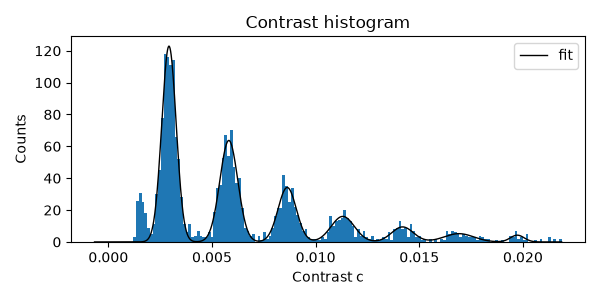
We model the histogram as a sum of bin-integrated Gaussians. The fitted peak centres (mu) are used as contrast values for the calibration fit.
bins = np.arange(-20, 660, 4) / contrast_slope_guess
initial_peaks = expected_masses_kDa / contrast_slope_guess

mpfit_calib = mp.distfit.fit(
    fitres_calib["contrasts"],
    bins=bins,
    initial_peaks=initial_peaks,
    include_background=False,
)

print("\nFitted peak centres (contrast):")
mpfit_calib.peaks[["mu", "sigma", "A"]]
Fitted peak centres (contrast):
Plot contrast histogram#
This is a useful sanity check: you should see distinct peaks and a reasonable fit overlay.
plt.figure(figsize=(6, 3))
plt.hist(fitres_calib["contrasts"], bins=bins, edgecolor="none")
plt.plot(mpfit_calib.model_x, mpfit_calib.model_y, color="black", lw=1, label="fit")
plt.xlabel("Contrast c")
plt.ylabel("Counts")
plt.title("Contrast histogram")
plt.legend()
plt.tight_layout()
Fit contrast-to-mass calibration#
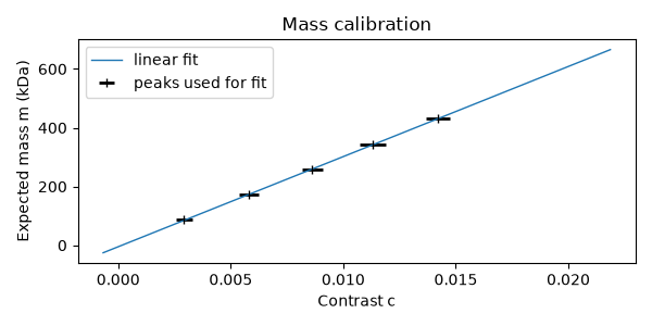
We fit a polynomial (default: linear) mapping contrast to mass (kDa). Often the lower-mass peaks are the cleanest, so we only use the first few for the fit.
n_values_for_fit = min(5, len(expected_masses_kDa), len(mpfit_calib.peaks))
calibration = mp.mass_calibration.fit(
    mpfit_calib.peaks["mu"][:n_values_for_fit],
    expected_masses_kDa[:n_values_for_fit],
)
print("\nFitted calibration (contrast -> mass, kDa):", calibration)
Fitted calibration (contrast -> mass, kDa): -4.98688693 + 30677.65217447·x
Update from existing calibration (mass-domain peaks)#
If you already have a previous calibration, measured peak positions may be in
mass units already. In that case, pass those values to fit
with input_unit='auto' (or 'mass') and provide the previous calibration
for inversion to contrast before fitting.
previous_calibration = (-5.2, 3.1e4)
measured_peak_masses_kDa = mp.mass_calibration.apply(
    mpfit_calib.peaks["mu"][:n_values_for_fit].to_numpy(),
    previous_calibration,
)
calibration_updated = mp.mass_calibration.fit(
    measured_peak_masses_kDa,
    expected_masses_kDa[:n_values_for_fit],
    input_unit="auto",
    reference_calibration=previous_calibration,
)
print("Updated calibration from mass-domain peak positions:", calibration_updated)
Updated calibration from mass-domain peak positions: -4.98688693 + 30677.65217447·x
Optionally, update the package wide defaults (massphoto.defaults.mass_calibration) with the fitted calibration.
calibration = mp.mass_calibration.fit(
    mpfit_calib.peaks["mu"][:n_values_for_fit],
    expected_masses_kDa[:n_values_for_fit],
    update_defaults=True,
)
Plot mass calibration#
This plot shows the fitted peak positions (with width estimates) and the resulting calibration curve.
plt.figure(figsize=(6, 3))
plt.errorbar(
    x=mpfit_calib.peaks["mu"][:n_values_for_fit],
    y=expected_masses_kDa[:n_values_for_fit],
    xerr=mpfit_calib.peaks["sigma"][:n_values_for_fit],
    fmt="|",
    color="black",
    capsize=0,
    linewidth=2,
    label="peaks used for fit",
)
x_fit = np.array([bins[0], bins[-1]], dtype=float)
plt.plot(x_fit, calibration(x_fit), lw=1, label="linear fit")
plt.xlabel("Contrast c")
plt.ylabel("Expected mass m (kDa)")
plt.title("Mass calibration")
plt.legend()
plt.tight_layout()
Apply calibration#
Apply the mass calibration to add a masses_kDa column to the fit results.
fitres_calib = mp.mass_calibration.apply(fitres_calib, calibration)

fitres_calib[["frame", "x", "y", "contrasts", "masses_kDa"]].head()
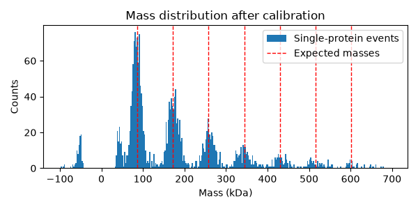
Mass distribution after calibration#
Finally, inspect the calibrated mass distribution. The expected ladder masses are shown as dashed vertical lines.
plt.figure(figsize=(6, 3))
plt.hist(
    fitres_calib["masses_kDa"],
    bins=np.arange(-100, 700, 2.5),
    edgecolor="none",
    label="Single-protein events",
)
for mass in expected_masses_kDa:
    plt.axvline(
        mass,
        color="red",
        ls="--",
        lw=1,
        label="Expected masses" if mass == expected_masses_kDa[0] else None,
    )
plt.xlabel("Mass (kDa)")
plt.ylabel("Counts")
plt.title("Mass distribution after calibration")
plt.legend()
plt.tight_layout()
Total running time of the script: (0 minutes 36.692 seconds)