Event rate and landing kinetics

This example demonstrates how to evaluate single-molecule binding kinetics over time:

1. Download an example movie and apply contrast-to-mass calibration.

2. Run detection and PSF fitting with massphoto.fit().

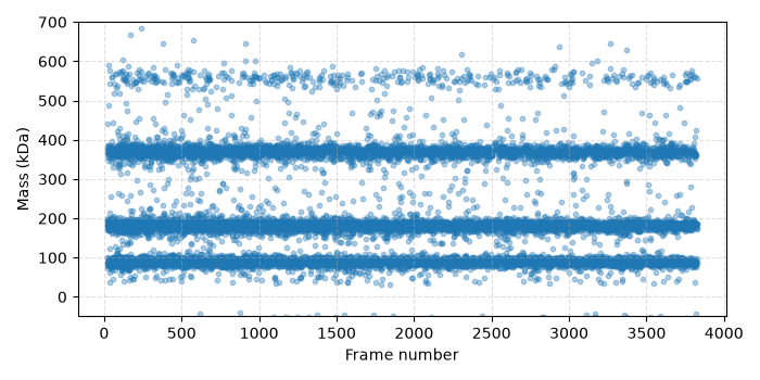
3. Filter events by fit quality using DataFrame.query().

4. Plot molecular mass vs. acquisition frame.

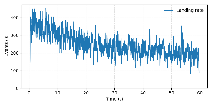
5. Compute and plot the event landing rate over time.

Imports and Setup

import matplotlib.pyplot as plt
import numpy as np
from zenodozipdownloader import ZenodoZipDownloader

import massphoto as mp

# Download example movie from Zenodo
files = ZenodoZipDownloader(
    doi="10.5281/zenodo.15800729",
    download_dir="example_data",
).download("Figure 2.zip/006_dynamin_6.mp")
if not files:
    raise RuntimeError(
        "Failed to download example data. Please download it manually from https://zenodo.org/record/15800729 "
        "or set path_movie to your own movie."
    )
path_movie = files[0]

Process the Movie

Configure mass calibration, disable progress bars for clean output in the docs, and run massphoto.fit():

mp.defaults.set("progress_bar", False)
mp.defaults.set("mass_calibration", (-5.2, 3.1e4))

movie, metadata = mp.read_movie(path_movie, convert_metadata=True)
fitres = mp.fit(movie)

Mass vs. Frame (Landing Events over Time)

A scatter plot of mass against frame reveals individual landing events as they occur. Stable bands confirm constant calibration and mass populations across the acquisition:

fig, ax = plt.subplots(figsize=(7, 3.5))
ax.scatter(fitres["frame"], fitres["masses_kDa"], s=10, alpha=0.35)
ax.set_xlabel("Frame number")
ax.set_ylabel("Mass (kDa)")
ax.set_ylim(-50, 700)
ax.grid(True, linestyle="--", alpha=0.4)
plt.tight_layout()
plt.show()

Event Landing Rate over Time

To detect surface saturation or sample depletion, it can be useful to inspect the landing rate of events over time.

window_size = 10  # frames
min_frame = int(fitres["frame"].min())
max_frame = int(fitres["frame"].max())
bins = np.arange(min_frame - 0.5, max_frame + 1)
counts, bin_edges = np.histogram(fitres["frame"], bins=bins)
bin_centers = (bin_edges[:-1] + bin_edges[1:]) / 2
counts_smooth = np.convolve(counts, np.ones(window_size) / window_size, mode="same")

# The metadata contains the effective frame rate, which allows us to define a time axis and convert counts per frame to counts per second:
time = bin_centers / metadata["framerate_effective"]
counts_smooth *= metadata["framerate_effective"]

fig, ax = plt.subplots(figsize=(7, 3.5))
ax.plot(time, counts_smooth, label="Landing rate")
ax.set_xlabel("Time (s)")
ax.set_ylabel("Events / s")
ax.set_ylim(bottom=0)
ax.grid(True, linestyle="--", alpha=0.4)
ax.legend(frameon=False)
plt.tight_layout()
plt.show()