Shot noise curve

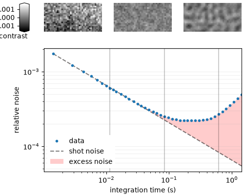
The shot noise curve is a practical tool for characterising the noise floor of a mass photometry measurement. It shows how the standard deviation of the ratiometric signal decreases as a function of the averaging window \(n_{avg}\).

In an ideal, shot-noise-limited measurement the standard deviation falls as \(1/\sqrt{n_{avg}}\). Any excess above this line indicates additional noise sources such as laser intensity fluctuations, mechanical vibrations, or sample drift.

This example computes the curve from scratch using massphoto.calc_ratiometric() and plots it on log-log axes together with the shot noise reference and the excess noise region.

Imports

import matplotlib.pyplot as plt
import numpy as np

import massphoto as mp

Download example data

We use a buffer (PBS) only measurement without protein landing events.

from zenodozipdownloader import ZenodoZipDownloader

files = ZenodoZipDownloader(
    doi="10.5281/zenodo.15800729",
    download_dir="example_data",
).download("Figure 4.zip/4a/PBS_4.mp")
if not files:
    raise RuntimeError(
        "Failed to download example data. Please download it manually from "
        "https://zenodo.org/record/15800729 or set path_movie to your own movie."
    )
path_movie = files[0]
print(f"Using movie: {path_movie}")

Using movie: /home/runner/work/massphoto/massphoto/docs/source/_examples/example_data/4a/PBS_4.mp

Read movie and extract frame rate

massphoto.read_movie() returns the raw pixel data and a metadata dictionary. Passing convert_metadata=True sets framerate_effective (frame rate after any pre-binning), which we use to label the x-axis in seconds.

movie, metadata = mp.read_movie(path_movie, convert_metadata=True)
fps = metadata["framerate_effective"]

# Crop to a spatial sub-region and limit frames to speed up the example
movie = movie[:5000, 10:30, 80:120]

print(f"Movie shape: {movie.shape}  dtype: {movie.dtype}")
print(f"Effective frame rate: {fps:.1f} Hz")

Movie shape: (5000, 20, 40)  dtype: uint16
Effective frame rate: 699.0 Hz

Compute the shot noise curve

For each averaging window size \(n_{avg}\) we:

1. Compute the full ratiometric movie with massphoto.calc_ratiometric().

2. Take the standard deviation of each valid frame over the spatial axes, then average across frames.

The averaging window sizes are generated with a log-spaced grid so that the curve is sampled evenly on the log-log plot. We cap \(n_{avg}\) at half the movie length to ensure there are always enough frames to compute the ratiometric signal.

navg_max = min(1000, movie.shape[0] // 2 - 1)
navgs = np.unique(np.logspace(0, np.log10(navg_max)).astype(int))

r_std_avg = np.zeros(navgs.size)

for idx, navg in enumerate(navgs):
    r = mp.calc_ratiometric(movie, navg, medfilt_kernel_size=0)
    r_std = np.std(r, axis=(1, 2))
    r_std = r_std[np.isfinite(r_std)]
    r_std_avg[idx] = np.mean(r_std)

Plot

The top row shows ratiometric frame thumbnails at three example integration times so you can see how the image improves as \(n_{avg}\) grows. The bottom panel shows the shot noise curve: the dashed black line is the theoretical \(1/\sqrt{n_{avg}}\) shot noise limit anchored to the first data point, and the red region highlights excess noise above that floor.

# Three navg values spread across the range for the thumbnails
frames_navgs = navgs[[len(navgs) // 6, len(navgs) // 2, len(navgs) * 5 // 6]]
nframes = len(frames_navgs)
frame_idx = movie.shape[0] // 2

fig = plt.figure(figsize=(5, 4))
gs = fig.add_gridspec(nrows=2, ncols=nframes, height_ratios=[1, 4], left=0.18, right=0.99, bottom=0.12, top=0.99)

ax_fr = [fig.add_subplot(gs[0, 0])]
for i in range(1, nframes):
    ax_fr.append(fig.add_subplot(gs[0, i], sharex=ax_fr[0], sharey=ax_fr[0]))

ax_curve = fig.add_subplot(gs[1, :])

cmax = 0.0016
for ax, navg in zip(ax_fr, frames_navgs):
    start = max(frame_idx - navg - 1, 0)
    r0 = mp.calc_ratiometric(movie[start : frame_idx + navg + 2], navg, medfilt_kernel_size=0)
    im = ax.imshow(r0[r0.shape[0] // 2], cmap="gray", vmin=-cmax, vmax=cmax)
    ax.axis("off")
    ax.set_xlabel(f"{navg / fps:.2g} s", fontdict={"fontweight": "light"})

ax_pos = ax_fr[0].get_position().bounds
cbaxes = fig.add_axes((0.08, ax_pos[1], 0.04, ax_pos[3]))
plt.colorbar(im, cax=cbaxes, extend="both")
cbaxes.yaxis.set_ticks_position("left")
cbaxes.set_xlabel("contrast", loc="right")
cbaxes.xaxis.set_label_coords(0.8, -0.1)

t = navgs / fps  # convert averaging window from frames to seconds

ax_curve.fill_between(
    t,
    r_std_avg[0] / np.sqrt(navgs),
    r_std_avg,
    color="r",
    alpha=0.2,
    edgecolor="none",
    label="excess noise",
)
ax_curve.loglog(t, r_std_avg[0] / np.sqrt(navgs), "--k", alpha=0.5, label="shot noise")
ax_curve.loglog(t, r_std_avg, ".", label="data")

# Mark the thumbnail integration times on the curve
for navg in frames_navgs:
    ax_curve.axvline(navg / fps, color="k", alpha=0.2)

ax_curve.set_xlim(right=t[-1])
ax_curve.grid(axis="y", visible=True, which="both", alpha=0.2)
ax_curve.set_xlabel("integration time (s)")
ax_curve.set_ylabel("relative noise")

handles, labels = ax_curve.get_legend_handles_labels()
ax_curve.legend(
    reversed(handles), reversed(labels), loc="lower left", facecolor="white", edgecolor="none", framealpha=1
)

plt.tight_layout()