Note
Go to the end to download the full example code.
Step-by-step pipeline#
This tutorial walks through each stage of the mass photometry analysis
pipeline individually, using the lower-level API instead of the high-level
massphoto.fit(). Exposing the intermediate results at every step
makes it easier to inspect, tune, and debug the analysis.
Imports#
import matplotlib.pyplot as plt
import numpy as np

import massphoto as mp
Download example data#
We use the same dynamin movie as in the other tutorials.
from zenodozipdownloader import ZenodoZipDownloader

files = ZenodoZipDownloader(
    doi="10.5281/zenodo.15800729",
    download_dir="example_data",
).download("Figure 2.zip/006_dynamin_6.mp")
if not files:
    raise RuntimeError(
        "Failed to download example data. Please download it manually from "
        "https://zenodo.org/record/15800729 or set path_movie to your own movie."
    )
path_movie = files[0]
print(f"Using movie: {path_movie}")
Using movie: /home/runner/work/massphoto/massphoto/docs/source/_examples/example_data/006_dynamin_6.mp
Step 1 — Read movie#
massphoto.read_movie() returns the raw pixel data as a NumPy array and a
metadata dictionary.
movie, metadata = mp.read_movie(path_movie, convert_metadata=True)
print(f"Movie shape: {movie.shape}  dtype: {movie.dtype}")

# Plot the middle frame as a quick sanity check
mid_idx = movie.shape[0] // 2
fig, ax = plt.subplots(figsize=(5, 5))
im = ax.imshow(movie[mid_idx], cmap="gray")
ax.set_title(f"Raw frame {mid_idx}")
ax.axis("off")
plt.colorbar(im, ax=ax, fraction=0.04, pad=0.04, label="Camera counts")
plt.tight_layout()
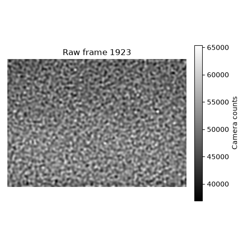
Movie shape: (3846, 166, 233) dtype: uint16
Step 2 — Drift correction#
Sample drift shifts individual frames relative to a reference, which
degrades both detection sensitivity and PSF fitting accuracy. We correct it
here using massphoto.correct_drift().
For more details on the drift correction step, including visualisation of per-frame drift, see Drift correction.
Step 3 — Ratiometric frames#
massphoto.calc_ratiometric() calculates a running relative change in intensity for each pixel.
This reveals transient contrast changes caused by molecules landing or leaving, while removing
static background. The function also subtracts a median-filtered background to further suppress
large-scale intensity variations.
movie_r = mp.calc_ratiometric(movie, medfilt_kernel_size=15)
print(f"Ratiometric movie shape: {movie_r.shape}  dtype: {movie_r.dtype}")

# Plot the same frame from the ratiometric movie
fig, ax = plt.subplots(figsize=(5, 5))
vmin, vmax = np.quantile(movie_r[mid_idx], [0.002, 0.998])
im = ax.imshow(movie_r[mid_idx], vmin=vmin, vmax=vmax)
ax.set_title(f"Ratiometric frame {mid_idx}")
ax.axis("off")
plt.colorbar(im, ax=ax, fraction=0.04, pad=0.04, shrink=0.8, label="Ratiometric contrast")
plt.tight_layout()
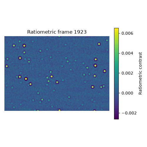
Ratiometric movie shape: (3846, 166, 233) dtype: float64
Step 4 — Filter maps#
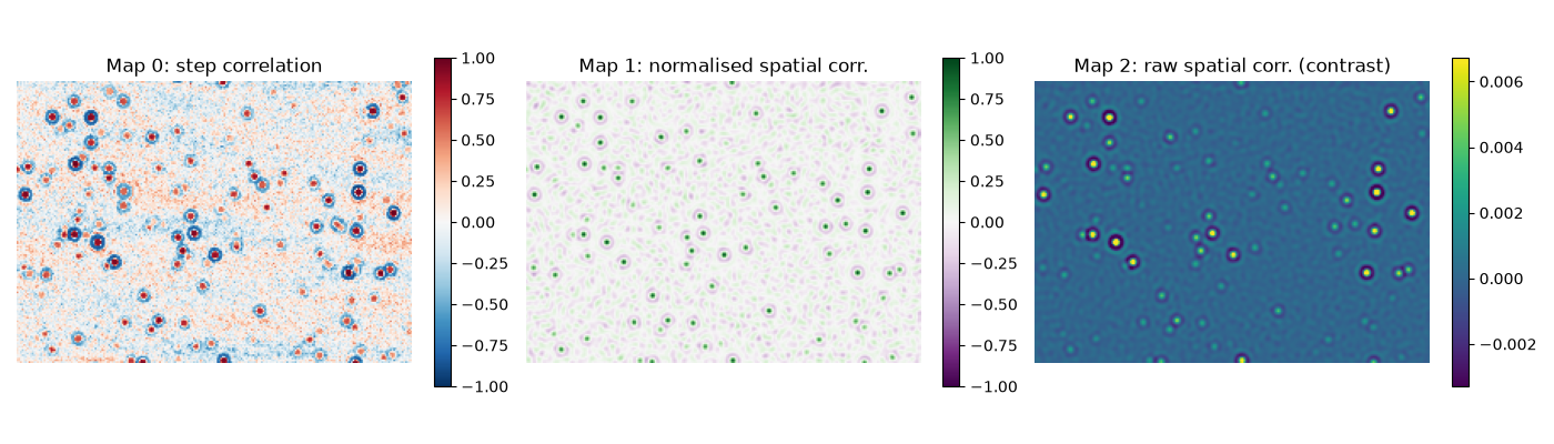
massphoto.detection.event_correlation_step() internally computes three maps
before calling massphoto.detect_on_map(). Here we compute them explicitly
so we can inspect each one.
With correlation_native_args=False (the default used by
massphoto.fit()), the step-correlation map is computed directly
from the raw (native) movie without any prior spatial filtering.
- Map 0 — Step correlation (temporal)
Normalised cross-correlation of the native intensity trace with a ±1 step template. Peaks where a molecule lands or leaves.
- Map 1 — Normalised spatial correlation
Cross-correlation of each ratiometric frame with a PSF kernel using
skimage.feature.match_template(), normalised per window. High where the frame contrast pattern matches the PSF shape.- Map 2 — Raw spatial correlation (contrast)
Unnormalised cross-correlation with the PSF kernel: proportional to the event contrast, so it scales with mass.
tcorr_map = mp.filter.step_correlation(movie)
ncorr_map, corr_map = mp.filter.correlation_map(movie_r)

# Plot one frame from each map side-by-side
frame = mid_idx
fig, axes = plt.subplots(1, 3, figsize=(14, 4))

im0 = axes[0].imshow(tcorr_map[frame], cmap="RdBu_r", vmin=-1, vmax=1)
axes[0].set_title("Map 0: step correlation")
plt.colorbar(im0, ax=axes[0], shrink=0.8, fraction=0.04)

im1 = axes[1].imshow(ncorr_map[frame], cmap="PRGn", vmin=-1, vmax=1)
axes[1].set_title("Map 1: normalised spatial corr.")
plt.colorbar(im1, ax=axes[1], shrink=0.8, fraction=0.04)

vmin, vmax = np.quantile(corr_map[frame], [0.002, 0.998])
im2 = axes[2].imshow(corr_map[frame], cmap="viridis", vmin=vmin, vmax=vmax)
axes[2].set_title("Map 2: raw spatial corr. (contrast)")
plt.colorbar(im2, ax=axes[2], shrink=0.8, fraction=0.04)

for ax in axes:
    ax.axis("off")
plt.tight_layout()
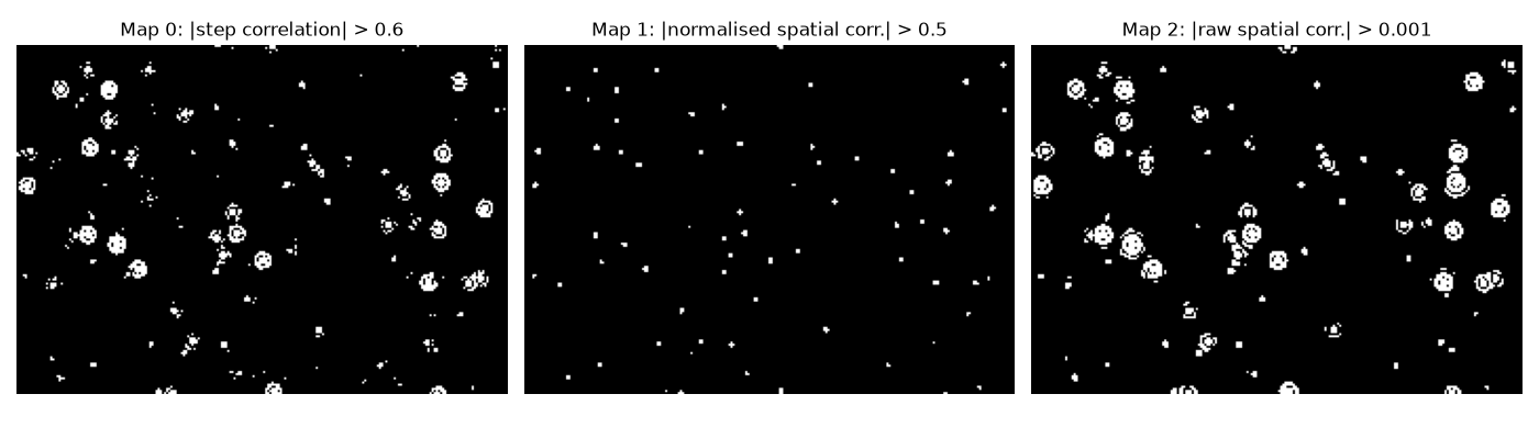
Taking the absolute value before thresholding, the binary detection maps for the thresholds used in the next step look like this:
thresholds = [0.6, 0.5, 0.001]
tcorr_map_bin = np.abs(tcorr_map) > thresholds[0]
ncorr_map_bin = np.abs(ncorr_map) > thresholds[1]
corr_map_bin = np.abs(corr_map) > thresholds[2]

fig, axes = plt.subplots(1, 3, figsize=(14, 4))
axes[0].imshow(tcorr_map_bin[frame], cmap="gray")
axes[0].set_title("Map 0: |step correlation| > 0.6")
axes[1].imshow(ncorr_map_bin[frame], cmap="gray")
axes[1].set_title("Map 1: |normalised spatial corr.| > 0.5")
axes[2].imshow(corr_map_bin[frame], cmap="gray")
axes[2].set_title("Map 2: |raw spatial corr.| > 0.001")
for ax in axes:
    ax.axis("off")
plt.tight_layout()
Step 5 — Detection#
massphoto.detect_on_map() finds local maxima that exceed the per-map
thresholds. The default thresholds from
massphoto.detection.event_correlation_step() are used here.
detections = mp.detect_on_map(
    (tcorr_map, ncorr_map, corr_map),
    thresholds=thresholds,
    threshold_absolute=True,
    threshold_distance_spat=3,
    min_distance_temp=10,
    position_map=2,
    contrast_map=2,
)
print(f"Detected events: {len(detections)}")

# Scatter plot of the first 1000 detections, colour-coded by frame number
n_show = min(1000, len(detections))
subset = detections.iloc[:n_show]

fig, ax = plt.subplots(figsize=(5, 5))
sc = ax.scatter(
    subset["x"],
    subset["y"],
    c=subset["frame"],
    cmap="viridis",
    s=20,
    alpha=0.8,
)
ax.set_xlim(0, movie.shape[2])
ax.set_ylim(movie.shape[1], 0)
ax.set_aspect("equal")
ax.set_xlabel("x (px)")
ax.set_ylabel("y (px)")
ax.set_title(f"First {n_show} detections (colour = frame)")
plt.colorbar(sc, ax=ax, shrink=0.4, label="Frame")
plt.tight_layout()
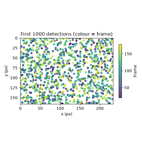
Detected events: 16592
Step 6 — PSF fitting#
massphoto.fit_event() fits a 2D PSF model to a thumbnail
around each detected position in the ratiometric movie, refining both the
position and the contrast estimate. The final count may be lower than the number of
detections because events too close to the movie border are excluded from fitting.
fitres = mp.fit_event(movie_r, detections)
print(f"Successfully fitted events: {len(fitres)}")

# Contrast distribution
bins = np.linspace(*np.quantile(fitres["contrasts"], [0.005, 0.995]), 100)
fig, ax = plt.subplots(figsize=(6, 3))
ax.hist(fitres["contrasts"], bins=bins, edgecolor="none")
ax.set_xlabel("Contrast")
ax.set_ylabel("Counts")
ax.set_title("Contrast distribution of fitted events")
plt.tight_layout()
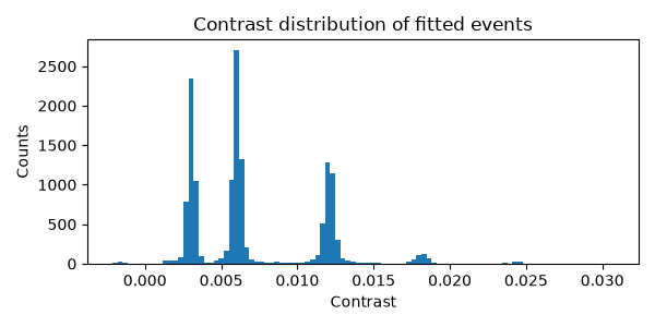
Successfully fitted events: 14626
Step 7 — Mass calibration and histogram#
Apply a contrast-to-mass calibration (see Mass calibration for how to obtain one) and fit a Gaussian mixture model to the resulting mass distribution.
mass_calibration = (-5.2, 3.1e4)  # (intercept, slope) — converts contrast to mass in kDa
fitres = mp.mass_calibration.apply(fitres, mass_calibration=mass_calibration)

histfit = mp.distfit.fit(
    fitres["masses_kDa"],
    bins=np.arange(-100, 700, 2.5),
    include_background=True,
)
histfit.peaks[["mu", "sigma", "A"]].round(2)
Plot the calibrated mass distribution and its fitted peaks.
fig, ax = plt.subplots(figsize=(6, 3))
ax.bar(histfit.bin_centers, histfit.counts, width=histfit.bin_widths, edgecolor="none", label="Data")
ax.plot(histfit.model_x, histfit.model_y, color="black", lw=1, label="Fit")
ax.set_xlabel("Mass (kDa)")
ax.set_ylabel("Counts")
ax.set_title("Mass distribution")
ax.legend()
plt.tight_layout()
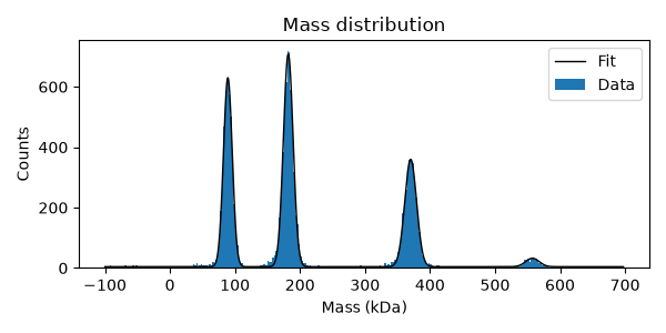
Total running time of the script: (1 minutes 2.966 seconds)