Mass distribution

This tutorial shows how to compute and fit mass distributions from a movie once a contrast-to-mass calibration is available:

1. Download an example movie.

2. Set a contrast-to-mass calibration.

3. Run detection + PSF fitting to obtain a table of event masses.

4. Fit peaks in the mass histogram and visualize the result.

Imports

We first import necessary packages and modules.

from pprint import pprint

import matplotlib.pyplot as plt
import numpy as np

Download example data

This tutorial uses a short example movie from Zenodo. You can replace this block with a direct file path once you have a local movie.

from zenodozipdownloader import ZenodoZipDownloader

import massphoto as mp

files = ZenodoZipDownloader(
    doi="10.5281/zenodo.15800729",
    download_dir="example_data",
).download("Figure 2.zip/006_dynamin_6.mp")
if not files:
    raise RuntimeError(
        "Failed to download example data. Please download it manually from https://zenodo.org/record/15800729 "
        "or set path_movie to your own movie."
    )
path_movie = files[0]

print(f"Using movie: {path_movie}")

Using movie: /home/runner/work/massphoto/massphoto/docs/source/_examples/example_data/006_dynamin_6.mp

Analyse with default parameters

Set mass calibration parameters. See the mass calibration example for how to obtain these from a calibration movie: Mass calibration.

# Disable progress bars for cleaner output in this tutorial
mp.defaults.set("progress_bar", False)

# Set contrast-to-mass calibration parameters (intercept, slope). Adjust to match your calibration.
mp.defaults.set("mass_calibration", (-5.2, 3.1e4))

# Run detection and fitting. Keep the ratiometric frames for inspecting events.
# Sequential execution limits peak memory while retaining those frames.
fitres, movie_r = mp.fit(path_movie, return_ratiometric=True, scheduler="synchronous")
fitres[["frame", "x", "y", "contrasts", "masses_kDa"]].head().round({"x": 2, "y": 2, "contrasts": 5, "masses_kDa": 1})

	frame	x	y	contrasts	masses_kDa
0	20	86.09	6.87	0.00343	101.2
1	20	165.06	72.34	0.00604	182.1
2	20	205.38	74.17	0.00648	195.8
3	20	124.95	80.87	0.00580	174.5
4	20	189.78	93.18	0.01202	367.4

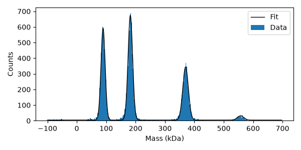
Fit mass distribution

histfit = mp.distfit.fit(fitres["masses_kDa"], bins=np.arange(-100, 700, 2.5), include_background=True)
histfit.peaks[["mu", "sigma", "A"]].round(2)

	mu	sigma	A
0	89.37	7.15	4199.50
1	182.20	7.82	5248.13
2	370.17	9.50	3235.14
3	557.33	10.71	290.48

Plot results

plt.figure(figsize=(6, 3))
plt.bar(histfit.bin_centers, histfit.counts, width=histfit.bin_widths, edgecolor="none", label="Data")
plt.plot(histfit.model_x, histfit.model_y, color="black", lw=1, label="Fit")
plt.xlabel("Mass (kDa)")
plt.ylabel("Counts")
plt.legend()
plt.tight_layout()

Analyse with custom parameters

# Read the movie
movie, metadata = mp.read_movie(path_movie, convert_metadata=True)


# Inspect the metadata
print("Metadata:")
pprint(metadata)

# Check default thresholds for detection
print("Default detection thresholds:", mp.defaults.get("event_correlation_step.thresholds"))

# We could adjust these if we want to be more or less sensitive, for all following analyses. For example:
# mp.defaults.set("event_correlation_step.thresholds", [0.5, 0.4, 0.001])

# Check default averaging window
print("Default navg:", mp.defaults.get("navg"))

# We could adjust the default like this:
# mp.defaults.set("navg", 5)


##
# We can also specify detection arguments here, which will only apply to this fit call.
fitres = mp.fit(
    movie,
    movie_correct_drift=True,
    ratiometric_args={
        "navg": 5,
    },
    detection_args={
        "thresholds": [
            0.5,  # temporal threshold
            0.4,  # spatial threshold
            0.001,  # contrast threshold
        ],
        # navg for the temporal filter (longer than navg for the ratiometric filter is often beneficial)
        "correlation_step_args": {"navg": 10},
    },
)

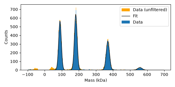
# We decreased the integration time and lowered the thresholds, which leads to more events being detected, but also more noise.
# To remove some of the noise, we can filter based on fit quality or mass uncertainty.
filter_str = "masses_kDa_se < 10 & r2_fit > 0.4"
histfit = mp.distfit.fit(
    fitres.query(filter_str),
    bins=np.arange(-100, 700, 2.5),
    initial_peaks=(90, 180, 360, 540),
    include_background=False,
)
histfit.peaks[["mu", "sigma", "A"]].round(2)

Metadata:
{'camera': 'GS3_U3_23S6M_C',
 'exposuretime': 7.646799087524414,
 'exposuretime_effective': 15.293598175048828,
 'exposuretime_unit': 'ms',
 'field_of_view': (11.7528, 16.4964),
 'field_of_view_unit': 'um',
 'framebinning': 2,
 'framerate': 128.20632934570312,
 'framerate_effective': 64.10316467285156,
 'framerate_unit': 'Hz',
 'image_shape': (166, 233),
 'instrument': 'Refeyn TwoMP',
 'pixelbinning': 6,
 'pixelsize': 0.0118,
 'pixelsize_effective': 0.0708,
 'pixelsize_unit': 'um'}
Default detection thresholds: (0.6, 0.5, 0.001)
Default navg: 10

	mu	sigma	A
0	89.72	8.04	4527.06
1	182.05	8.22	5284.42
2	369.90	9.73	3245.49
3	557.76	12.82	372.53

Compare the unfiltered distribution, selected events, and fitted peaks.

plt.figure(figsize=(6, 3))
plt.hist(fitres["masses_kDa"], bins=histfit.bin_edges, edgecolor="none", facecolor="orange", label="Data (unfiltered)")
plt.bar(histfit.bin_centers, histfit.counts, width=histfit.bin_widths, edgecolor="none", label="Data")
plt.plot(histfit.model_x, histfit.model_y, color="black", lw=1, label="Fit")
plt.xlabel("Mass (kDa)")
plt.ylabel("Counts")
plt.legend()
plt.tight_layout()