Custom detection function

This tutorial shows how to implement a custom detection function and use it with massphoto.fit():

1. Download an example movie.

2. Set a contrast-to-mass calibration.

3. Define a custom detection function using a Gaussian Laplace filter.

4. Run detection + PSF fitting with the custom function.

5. Visualize the mass distribution and the detection map values.

Imports

We first import necessary packages and modules.

import matplotlib.pyplot as plt
import numpy as np
import scipy as sp

import massphoto as mp

Download example data

This tutorial uses a short example movie from Zenodo. You can replace this block with a direct file path if you have a local movie.

from zenodozipdownloader import ZenodoZipDownloader

files = ZenodoZipDownloader(
    doi="10.5281/zenodo.15800729",
    download_dir="example_data",
).download("Figure 2.zip/006_dynamin_6.mp")
if not files:
    raise RuntimeError(
        "Failed to download example data. Please download it manually from https://zenodo.org/record/15800729 "
        "or set path_movie to your own movie."
    )
path_movie = files[0]

print(f"Using movie: {path_movie}")

Using movie: /home/runner/work/massphoto/massphoto/docs/source/_examples/example_data/006_dynamin_6.mp

Set up calibration

Set mass calibration parameters. See the mass calibration example for how to obtain these from a calibration movie: Mass calibration.

# Disable progress bars for cleaner output in this tutorial
mp.defaults.set("progress_bar", False)

# Set contrast-to-mass calibration parameters (intercept, slope). Adjust to match your calibration.
mp.defaults.set("mass_calibration", (-5.2, 3.1e4))

Define a custom detection function

A custom detection function must accept one or two input movie as np.ndarray and return a DataFrame of detected events. Annotating the movie argument with massphoto.NativeMovie or massphoto.RatiometricMovie tells the pipeline which movie representation to pass; the values themselves are plain np.ndarray instances. Similarly, massphoto.EventList annotates the output but is just a pd.DataFrame. Any additional parameters can be exposed as keyword arguments which can be passed via detection_args.

Here we use scipy.ndimage.gaussian_laplace() as the spatial filter. You can swap in any filter that returns an array of the same shape.

def custom_detect(
    movie: mp.RatiometricMovie,
    sigma: float = 2.5,
    threshold: float = 1e-4,
    **kwargs,
) -> mp.EventList:
    """Detect events using a Gaussian Laplace filter on the ratiometric movie.

    Applies :func:`scipy.ndimage.gaussian_laplace` frame-by-frame and then
    calls :func:`massphoto.detect_on_map` on the resulting filter response.

    Parameters
    ----------
    movie : mp.RatiometricMovie
        Ratiometric movie array (np.ndarray: T x H x W). Using this type annotation
        ensures that the ratiometric movie is passed to the function by the pipeline.
    sigma : float, optional
        Standard deviation of the Gaussian kernel. Default is 2.5.
    threshold : float, optional
        Absolute detection threshold on the Gaussian Laplace response.
        Default is 1e-4.
    **kwargs
        Additional keyword arguments forwarded to
        :func:`scipy.ndimage.gaussian_laplace`.

    Returns
    -------
    mp.EventList
        DataFrame of detected events with columns ``frame``, ``y``, ``x``,
        and map values.

    Notes
    -----
    Custom detection functions must handle empty input (``movie.shape[0] == 0``)
    correctly, because the parallel pipeline calls them with a zero-frame chunk
    to infer the output schema before processing real data. Any filter or helper
    used inside the function must therefore also tolerate empty arrays.
    :func:`massphoto.filter.stack_apply_filter` satisfies this requirement.
    """
    detection_map = mp.filter.stack_apply_filter(sp.ndimage.gaussian_laplace, movie, sigma=sigma, **kwargs)

    detections = mp.detect_on_map(
        (detection_map, movie),
        thresholds=[threshold, 0.0],
        threshold_absolute=True,
        min_distance_temp=15,
        min_distance_spat=9,
        position_map=0,
        contrast_map=1,
        output_map_values=True,
    )
    return detections

Run detection and fitting

Pass the custom function via detection_func. Any parameters it exposes can be tuned through detection_args.

fitres = mp.fit(path_movie, detection_func=custom_detect, detection_args={"sigma": 2.5, "threshold": 1e-4})

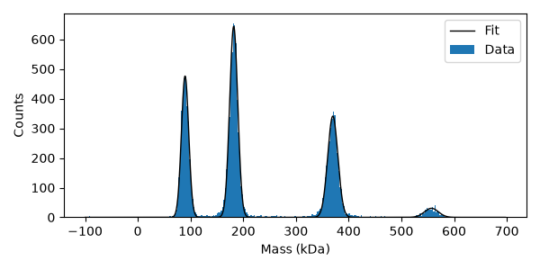
# Fit mass distribution
histfit = mp.distfit.fit(fitres["masses_kDa"], bins=np.arange(-100, 700, 2.5), include_background=False)
histfit.peaks[["mu", "sigma", "A"]].round(2)

	mu	sigma	A
0	89.69	6.90	3294.80
1	181.95	7.68	4954.61
2	369.94	9.67	3305.41
3	557.02	13.31	407.40

Plot results

plt.figure(figsize=(6, 3))
plt.bar(histfit.bin_centers, histfit.counts, width=histfit.bin_widths, edgecolor="none", label="Data")
plt.plot(histfit.model_x, histfit.model_y, color="black", lw=1, label="Fit")
plt.xlabel("Mass (kDa)")
plt.ylabel("Counts")
plt.legend()
plt.tight_layout()

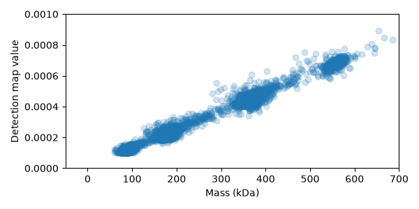
Detection map value vs mass

The Gaussian Laplace response scales with event contrast (and therefore mass), so larger events are easier to detect above the threshold. The default filters are normalised to have a more mass-independent response.

We have passed output_map_values=True to the detection function which lets us inspect the detection map values for each event. Here we plot these values against the fitted masses to see how they correlate.

plt.figure(figsize=(6, 3))
plt.scatter(fitres["masses_kDa"], fitres["map_0"], alpha=0.2)
plt.xlim(-50, 700)
plt.ylim(0, 1e-3)
plt.xlabel("Mass (kDa)")
plt.ylabel("Detection map value")
plt.tight_layout()